Quantum Deep Learning

Introduction

Today we are going to dive straight into one of the most complex and almost unimaginably perplexing fields of research currently being undertaken across the world today – that of quantum computing and its incredible potential to not just transform but introduce a complete paradigm shift in the way computers store and process information. In this article, we will be looking at how researchers are combining quantum computing with deep learning to reduce the time required to train a neural network, and by doing so introducing an entirely new framework for deep learning and performing underlying optimisation.

A Prediction

I am often asked by my clients what the future could look like. And I often include quantum computing in my response. Though it sounds like something from science fiction, researchers at companies like IBM and Google are actively transforming it from science fiction to science reality! I predict that the next decade will see the introduction of the first fully verified 100-qubit quantum chip. And when we talk about transformation in the 2030s, we will be talking about quantum computing-driven transformation and the exploitation of commercial quantum computing systems.

Artificial Neural Networks

In this section, we will briefly revisit the concept of the artificial neuron and the perceptron, before introducing how researchers are mimicking it on an actual real-world quantum processor! Recall that the core concepts of a natural neuron can be generalized into components of a signal processing system. In this general signal processing system, the signals received by natural dendrites can be modelled as inputs. The nucleus can be thought of as a central processing unit that collects and aggregates the inputs and, depending on the net input magnitude and an activation function, transmits outputs along the axon. This general signal processing system, modelled on a natural neuron, is called an artificial neuron and is illustrated below.

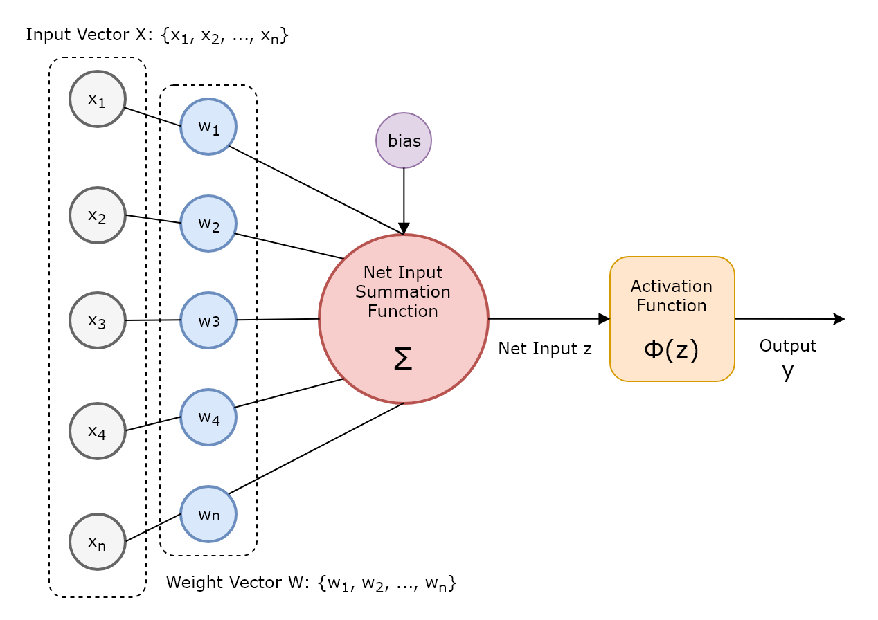
In the artificial neuron, weights can amplify or attenuate signals and are used to model the established connections to other neurons as found in the natural world. By changing the weight vectors, we can effect whether that neuron will activate or not based on the aggregation of input values with weights, called the weighted or net input z.

Once the weighted input plus a bias is calculated, the activation function is used to determine the output of the neuron and whether it activates or not. To make this determination, an activation function is typically a non-linear function bounded between two values, thereby adding non-linearity to artificial neural networks (ANN). As most real-world data tends to be non-linear in nature when it comes to complex use cases, we require that ANNs have the capability to learn these non-linear concepts or representations. This is enabled by non-linear activation functions, such as the sigmoid function. A sigmoid function is a non-linear mathematical function that exhibits a sigmoid curve, and often refers to the sigmoid or logistic function. In this case, the sigmoid activation function is bounded between 0 and 1 and is smoothly defined for all real input values, making it a better choice of activation function than say a basic Heaviside step function. This is because, unlike the Heaviside step function, non-linear activation functions can distinguish data that is not linearly separable, such as image and video data.

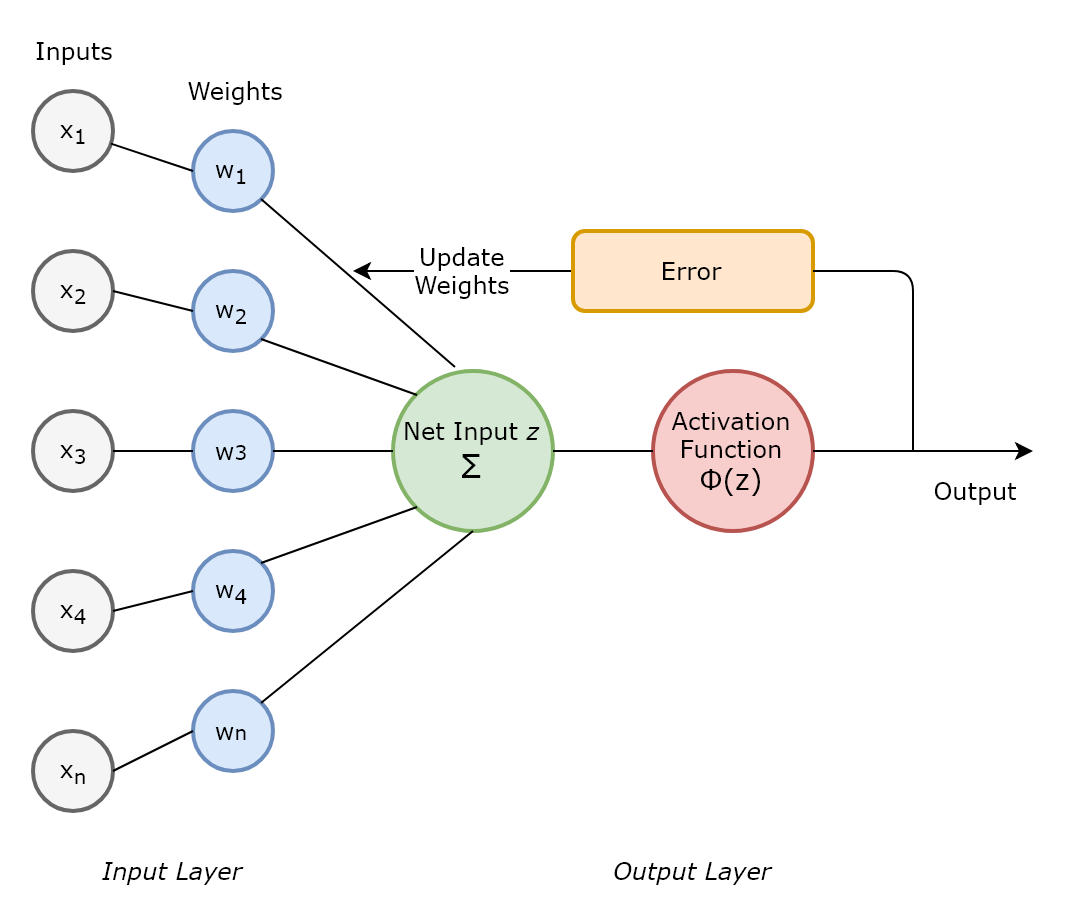
In the single-layer perceptron, an optimal set of weight coefficients are derived which, when multiplied by the input features, determines whether to activate the neuron or not. Initial weights are set randomly and, if the weighted input results in a predicted output that matches the desired output, then no changes to the weights are made. If the predicted output does not match the desired output, then weights are updated to reduce the error. This process is known as the perceptron learning rule.

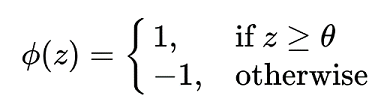
In this case, the activation function used is the Heaviside step function, whereby if the net input z, as defined above, is greater than a defined threshold theta, we predict "1" (positive class), else we predict "-1" (negative class).

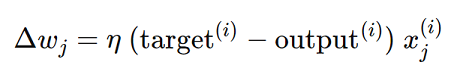
And the value by which to update the weights, where the Greek letter eta denotes the learning rate (a constant between 0 and 1), is computed using the following learning rule:

Quantum Computing and the Qubit

One of the limitations of this simple perceptron is that they are limited to when the classes are linearly separable. Furthermore when implemented in multi-layer perceptron architectures, as the number of neurons increase, so does the computational complexity.

Most implementations of artificial neural networks today are processed as a series of algorithms consolidated in a layer of software running on top of conventional hardware forming part of a distributed cluster. To improve performance even further, dedicated GPU clusters can be provisioned, significantly reducing training times. However, even this will pale into comparison when benchmarked against future quantum processors.

Researchers today are designing physical neural networks where the entire hardware itself represents an artificial neuron, as opposed to layers of software running on conventional hardware. And even more astonishingly, “qubit neurons” have already been created where the qubit itself acts as an individual neuron!

So what is a qubit? I must confess that I am no physicist and that most of the theoretical concepts in the weird and wonderful world of quantum physics are far beyond my understanding! However, using my 3rd year undergraduate notes from my Quantum Mathematics module……

To understand what a qubit is, let us first revisit those fundamental building blocks of traditional computers – bits. A bit represents a single binary value – it can either be 0 or 1 and are designed to store data and enable the execution of instructions, with 8 bits forming 1 byte. Using 8 bytes for example, or 64 bits, one can store an integer up to the value of 2 ^ 64 – 1 (try typing that into your calculator and see what you get!). So bits can only ever take the value of 0 and 1 at any one time. They can never be both at the same time. In other words, bits, and the systems they help to form, are always in a discrete and stable state.

Quantum mechanics on the other hand allows for systems to be in a state of quantum superposition, that is it may be in multiple states at the same time. Going back to our concept of the bit, this means that if:

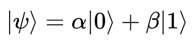
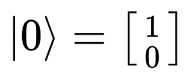
|0⟩ denotes the quantum state which, when measured, results in the classical equivalent of 0, and

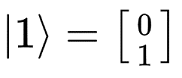
|1⟩ denotes the quantum state which, when measured, results in the classical equivalent of 1, then the state of a quantum bit (or qubit) is described by:

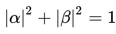
where the Greek letters alpha and beta are complex numbers satisfying:

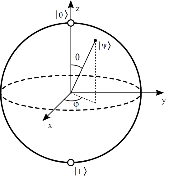
One way to visualise this is to imagine a sphere, as illustrated below. Classical bits can take the values of either 0 or 1 at any one time, and are represented by the poles of the sphere. Qubits on the other hand, because they can exist in a state of quantum superposition, can be thought of as a unit vector that can access any part of the sphere, whereas classical bits are confined to the poles.

In quantum physics, a quantum system can exist in a state of superposition until such time that it is measured. As soon as it is measured, the system is in a measured state, meaning that any future measurements will return the exact same value. In the context of the quantum bit, measuring its state (provided by the equation above) will result in:

|0⟩ with a probability of |α|² , and

|1⟩ with a probability of |β|²

Using linear algebra and vector notation, we can say that the state of a quantum bit, as described above, can be represented as a unit vector [alpha, beta] in a 2D complex vector space, as a linear superposition of the following basis vectors, or indeed any linearly independent vector pairs.

Quantum Entanglement

Now that we have an understanding of what a quantum bit is, another phenomenon that exists within quantum systems is that of quantum entanglement. Quantum entanglement describes the scenario whereby you cannot describe the quantum state of a particle independent of its wider system, even if those particles are separated by large distances. In other words, there is some quantum-level correlation between seemingly independent particles.

In the context of the quantum bit, an n-qubit system can exist in any superposition of its 2^n basis states. In a 2-qubit system, measuring the first qubit automatically determines the second qubit. This is a mind-boggling characteristic of quantum systems, and its application to quantum bits means that there exists correlation between qubits that is not possible between classical bits. This therefore means that quantum computers have the ability to perform complex calculations that would take classical computers thousands of years by the fact that measuring one qubit automatically determines another, significantly reducing processing times!

Qubit Neurons

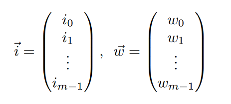
Let us now return to find out how researchers are actively using quantum bits to act as individual neurons. Given an N-qubit system, the classical m-dimensional input and weight vectors feeding a perceptron can be defined as m = 2^N, taking binary values of either -1 or 1. The quantum states of the N qubits can therefore be defined using this m-dimensional input vector with m coefficients. Given input and weight vectors i and w limited to the values -1 or 1 as follows:

Then the two quantum states can be defined as follows:

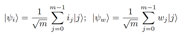
This equation can then be used to describe all possible states of the single qubits, in either |0⟩ or |1⟩ . Using the equation above as a basis from which to model a classical perceptron on a quantum processor, researchers have been able to experimentally demonstrate a working quantum perceptron on a 5-qubit IBM cloud-based quantum processor that has been able to classify simple and linearly separable patterns! This is remarkable, and clearly demonstrates that quantum physics and quantum computing, along with its inherent principles of quantum superposition and mind boggling quantum entanglement, is a physical reality!

The Future

Though quantum computing is a physical reality today, it is still some years away from being able to compete with, and thereafter quickly surpass, classical computers. However when that time comes, it will herald a paradigm shift in the complexity of processing that computers will be able to undertake and the amount of time in which they will be able to do it in. Furthermore, it will herald an extraordinary evolution in artificial intelligence where quantum computing will be unified with deep learning, leading to artificial cognitive systems comparable to that of natural intelligence.

Further Reading

• Quantum Neural Networks
• Machine Learning and Quantum Computing
• IBM Q Experience - Cloud based Quantum Processor
• Quantum Bit
• Quantum Superposition
• Quantum Entanglement